LBVH-As easy as possible

This blog post aims how I simplified Z-Order Curve based Linear Bounding Volume Hierarchy and implemented it via CPU (GPU based implimentation becomes lot more easier to understand afterwards).

What is LBVH exactly?

Lauterbach et al. [LGS∗ 09] proposed a way to construct a BVH tree by sorting input primitives along a space filling curve, bringing from 3D to 1D. The Idea was to construct special key values called Morton-Code from 3D Coordinates of every primitive, making them leaf nodes and build a tree on top of it. In 2012, Tero Karras improved the proposed paper by converting Top-down tree construction to bottom-up and node prediction so that it can be constructed in parallel inside a GPU.

Assuming you are here just for extremely simple form of Fast and Simple Agglomerative LBVH Construction, we will only focus on constructing the tree over CPU on single thread and no node prediction. It is highly recommended to read the paper at (download link) and blog post Thinking Parallel, Part III: Tree Construction on the GPU, NVIDIA Developer Blog.

Exploring Morton Codes

Mr. Asger Hoedt has a very good blog post at Morton Codes | Asger Hoedt.

However if would still recommend you to skim over my understandings.

Morton codes provide a way to represent multidimensional data to one dimension without affecting data’s relative position with respect to other data members.

Lets take an example shall we

You have many points or many spheres and we have to do a ray traversal over it, but before all that we have to construct the tree itself. How do we construct the tree, we need a way to represent it so that we can predict where the desired data may lie, for that we need to sort it, but how do we sort it. Let’s discuss how a typical bounding volume hierarchy looks like:

• take the array of primitives, split it in half into 2 teams with one that lies left of the yz plane and other right.
• Now split these slices into 2 teams again (inside slice/group’s own bounding box) along xz plane this time. Then again in xy plane and so on until you have individuals in every team.
• Good you have a sorted array create a tree on top of it while inserting a parent node at every split.

But everything is well and good but you might have noticed it to be slow, yeah tree construction will take time but as the gains greater much greater especially considering 10s of 1000s of ray intersection or collision checks or data checks it is bearable, however where does Morton codes magic comes in you ask. Well glad you thought, here comes the Morton code, we can do all of the above task in a single sort and save a ton on performance along the way while tree construction by rather than sorting by individual coordinate one at a time along each axis, construct a Morton code of each primitive and sort them in one go.

Sounds cool right, so well how does it work.

We know that computers represent numbers in binary so differing bit can split sections in 2, so what we can do is - according to decimal point we can add zeros and arrange them. Now the obstacles that are 1st one is we have a limited no. of fields or bits(in Morton code) to work with so we have to sacrifice accuracy with minimum effect 2nd which many of you guessed how floats are actually stored inside a 32-bit container. Floats (and doubles) are not your regular integer like containers, you can explore this on your own by the way (IEEE-754). Back to the topic, so we’re gonna have to arrange them, initially we could do is drag every primitive inside (0,0,0) to (1,1,1) range, steps are pretty simple find bounding box of entire scene, subtract min-point from every primitives transform, scale it down by right amount.

Scene AABB {xs1 , ys1 , zs1}, {xs2, ys2 , zs2}

same goes for y & z.

Now that every coordinate is within ∈ [0 1]. We have to only worry about what comes after the decimal point. Now watch which size of key(Morton code) you want to construct, is it 32-bit(suggested for small scene with less no. of artifacts) or 64-bit (for larger no. of artifacts) or you can go even crazy with even larger sizes like uint32_t[3] etc. Lets say you took 32-bit then 32/3 ~ 10.6 or 11 + 11 + 10 for x,y,z channel.

Now on to the 2nd obstacle that is floats and its encoding, well the thing is - you don’t have to worry about it, what we can instead of resolving mantissa(of floats) is:

// Since we have 10~11 bits to process for each coordinate
uint16_t[3] float_to_uint16coord = {
    uint16_t(double(newPt.x)*std::numeric_limits<uint16_t>::max), … };

now start from most to least significant bit (left to right) and create the Morton code, well actually you can find many Morton code generation references online.

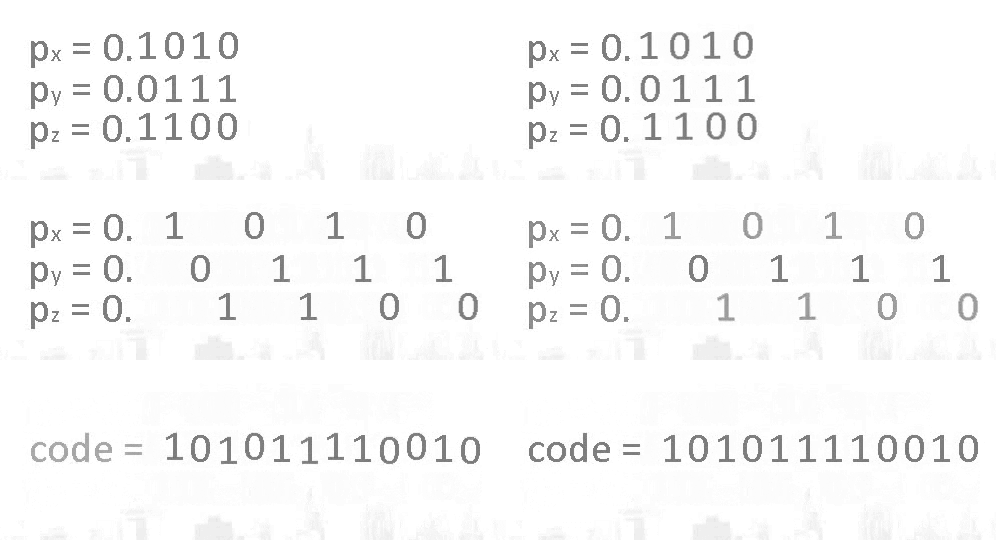
This article explains Morton code encoding and decoding much better than I can possibly could.

TIP: instead of std::numeric_limits<uint16_t>::max you can use two 11 bits and one 10 bit, this way you can sort faster, similarly for 64 bit Morton code instead of std::numeric_limits<uint32_t>::max you can use two 21 bit and one 22 bit for speed.

Well good job, now that we have Morton code, left to do is sort the primitives then create a tree out of it.

// Sorting is pretty easy (treat this as refrence as your implimentation will vary)
struct Key
{
	uint32_t MortonCode;
	uint32_t NodeID; // identifier for internal nodes
};
std::sort (keys.begin (), keys.end (),
   [&](Key a, Key b) -> bool {
      if (a.MortonCode == b.MortonCode) { // duplicate cases
	   glm::vec3 A = primitives_BBs[a.NodeID].second - primitives_BBs[a.NodeID].first;
	   glm::vec3 B = primitives_BBs[b.NodeID].second - primitives_BBs[b.NodeID].first;
	   return glm::dot (A, A) < glm::dot (B, B);
      }
   return a.MortonCode < b.MortonCode;
});

As For creating tree, well its also easy however there’s a catch I didn’t do it the way described by Karras in the paper. Although idea is the same but I do it differently (otherwise why would I write a blog about it).

First reserve tree container(or wherever you are storing nodes) to 2*n – 1, where n is no. of primitives.

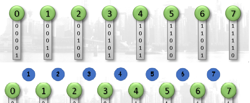
The good thing about this type of tree is the presence of exact n – 1 no. internal nodes, and only leaf node carry primitive data (however every node carries effective BB encompassing its children).

For every internal node we use ‘☊’ neighbouring leaf node’s uncommon most significant bit, then these internal are pushed to a queue from lowest to highest (of the uncommon most significant bit position). It checks the neighbour leaf, for right link check whether right neighbouring leaf has parents, if yes keep climbing up until you find orphan node, then adopt as left child, repeat this for right child again, using these children find encompassing Bounding box, move to the next in line. Ultimately root node will carry scene’s bounding box. Superb you now have your LBVH.

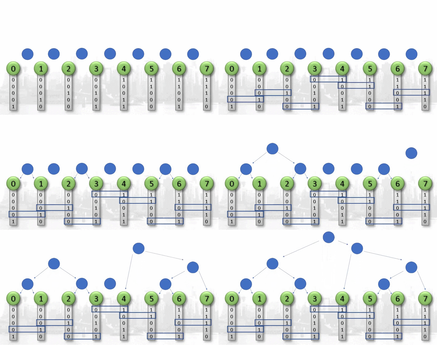
Note: when performing over multiple cores, instead of checking for parents, the future parents data can directly be inferred from bit differences among the region (this can be another topic for future discussions). All in all, as an over view of steps: Create Array of Leaf Nodes with their BB and NULL child Generate Morton code for these leaf nodes (I like to use mid-point of BB). Sort this array.

• Resize node array to 2n-1
• Create another array of size n–1 (for highest uncommon upper bit, corresponding to every internal node).
• Sort it from low to high with key: highest uncommon upper bit.
• Traverse this array to push internal nodes into a queue (of pointers to internal nodes).
• Repeat while queue is not empty - Pop the queue, solve the node for left and right child, calc new BB, link parent and children.
• Optional: since I use it for raytracing, collision detection etc. so before sending it over to the GPU, I recreate buffer with top(root is the last node that was pushed inside node array) to bottom traversal over the tree thus data becomes nice and clean to work with.

[LGS∗09] LAUTERBACH C., GARLAND M., SENGUPTA S., LUEBKE D., MANOCHA D.: Fast BVH construction on GPUs. Computer Graphics Forum 28, 2 (2009), 375–384.